
Want to share your content on R-bloggers? click here if you have a blog, or here if you don’t.
Reposted from the original at https://blog.stephenturner.us/p/uv-part-3-python-in-r-with-reticulate.
Two demos using Python in R via reticulate+uv: (1) Hugging Face transformers for sentiment analysis, (2) pyBigWig to query a BigWig file and visualize with ggplot2.
—
This is part 3 of a series on uv. Other posts in this series:
-
This post
-
Coming soon…
Python and R
I get the same question all the time from up and coming data scientists in training: “should I use Python or R?” My answer is always the same: it’s not Python versus R, it’s python and R — use whatever tool is best for the job. Last year I wrote a post with resources for learning Python as an R user.
“The best tool for the job” might require multilingual data science. I’m partial to R for data manipulation, visualization, and bioinformatics, but Python has a far bigger user base, and best to not reinvent the wheel if a well-tested and actively developed Python tool already exists.
Python in R with reticulate and uv
If I’m doing 90% of my analysis in an R environment but I have some Python code that I want to use, reticulate makes it easy to use Python code within R (from a script, in a RMarkdown/Quarto document, or in packages). This helps you avoid switching contexts and exporting data between R and Python.
You can import a Python package, and call a Python function from that package inside your R environment. Here’s a simple demo using the listdir() function in the os package in the Python standard library.
library(reticulate)
os <- import("os")
os$listdir(".")
Posit recently released reticulate 1.41 which simplifies Python installation and package management by using uv on the back end. There’s one simple function: py_require() which allows you to declare Python requirements for your R session. Reticulate creates an ephemeral Python environment using uv. See the function reference for details.
Demo 1: Hugging Face transformers
Here’s a demo. I’ll walk through how to use Hugging Face models from Python directly in R using reticulate, allowing you to bring modern NLP to your tidyverse workflows with minimal hassle. The code I’m using is here as a GitHub gist.
R has great tools for text wrangling and visualization (hello tidytext, stringr, and ggplot2), but imagine we want access to Hugging Face’s transformers library, which provides hundreds of pretrained models, simple pipeline APIs for things like sentiment analysis, named entity recognition, translation, or summarization.1 Let’s try running sentiment analysis with the Hugging Face transformers sentiment analysis pipeline.
First, load the reticulate library and use py_require() to declare that we’ll need PyTorch and the Hugging Face transformers library installed.
library(reticulate)
py_require("torch")
py_require("transformers")
Even after clearing my uv cache this installs in no time on my MacBook Pro.
Installed 23 packages in 411ms
Next, I’ll import the Python transformers library into my R environment, and create a object to use the sentiment analysis pipeline. You’ll get a message about the fact that you didn’t specify a model so it defaults to a DistilBERT model fine tuned on the Stanford Sentiment Treebank corpora.
transformers <- import("transformers")
analyzer <- transformers$pipeline("sentiment-analysis")
We can now use this function from a Python library as if it were an R function.
analyzer("It was the best of times")
The result is a nested list.
[[1]]
[[1]]$label
[1] "POSITIVE"

[[1]]$score
[1] 0.9995624
How about another?
analyzer("It was the worst of times")
Results:
[[1]]
[[1]]$label
[1] "NEGATIVE"

[[1]]$score
[1] 0.9997889
Let’s write an R function that gives us prettier output. This will take text and output a data frame indicating the overall sentiment and the score.
analyze_sentiment <- function(text) {
  result <- analyzer(text)[[1]]
  tibble(label = result$label, score = result$score)
}
Let’s try it out on a longer passage.
analyze_sentiment("it was the age of wisdom, it was the age of foolishness, it was the epoch of belief, it was the epoch of incredulity, it was the season of Light, it was the season of Darkness, it was the spring of hope, it was the winter of despair")
The results:
     label     score
1 NEGATIVE 0.5121167
Now, let’s create several text snippets:
mytexts <- c("I love using R and Python together!",
             "This is the worst API I've ever worked with.",
             "Results are fine, but the code is a mess",
             "This package manager is super fast.")
And using standard tidyverse tooling, we can create a table showing the sentiment classification and score for each of them:
library(dplyr)
library(tidyr)
tibble(text=mytexts) |>
  mutate(sentiment = lapply(text, analyze_sentiment)) |>
  unnest_wider(sentiment)
The result:
# A tibble: 4 × 3
  text                                         label    score
  <chr>                                        <chr>    <dbl>
1 I love using R and Python together!          POSITIVE 1.00
2 This is the worst API I've ever worked with. NEGATIVE 1.00
3 Results are fine, but the code is a mess     NEGATIVE 0.999
4 This package manager is super fast.          POSITIVE 0.995
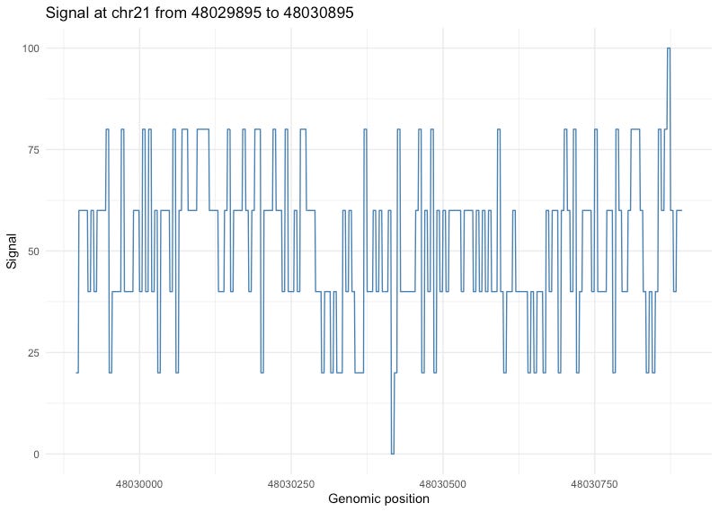
Demo 2: pyBigWig to query a BigWig file
This example demonstrates using pyBigWig to query a BigWig file in R for downstream visualization with ggplot2. All the code is here as a GitHub Gist.
First, let’s get this example BigWig file:
x <- "http://genome.ucsc.edu/goldenPath/help/examples/bigWigExample.bw"
download.file(x, destfile = "bigWigExample.bw", mode = "wb")
Now let’s load reticulate and use the pyBigWig library:
library(reticulate)
py_require("pyBigWig")
pybw <- import("pyBigWig")
Now let’s open that example file, look at the chromosomes and their lengths, then query values near the end of chromosome 21.
# Open a BigWig file
bw <- pybw$open("bigWigExample.bw")

# Get list of chromosomes
chroms <- bw$chroms()
print(chroms)

# Query values near the end of chromosome 21
chrom <- "chr21"
start <- chroms[[1]]-100000L
end <- start+1000L

# Get values (one per base)
values <- bw$values(chrom, start, end)

# Close the file
bw$close()
Finally, we can put the results into a data frame and plot it with ggplot2:
# Wrap into data frame
df <- data.frame(position = start:(end - 1),
                 signal = unlist(values))

# Plot the result
library(ggplot2)
ggplot(df, aes(x = position, y = signal)) +
  geom_line(color = "steelblue") +
  theme_minimal() +
  labs(title = paste("Signal at", chrom, "from", start, "to", end),
       x = "Genomic position",
       y = "Signal")
Here’s the resulting plot:
Until recently support for this kind of tooling in R was minimal or non-existent. With new tools like ellmer, mall, and many others now on the scene, R is catching up quickly with the Python ecosystem for developing with LLMs and other AI tools. See my previous post demonstrating some of these tools.
R-bloggers.com offers daily e-mail updates about R news and tutorials about learning R and many other topics. Click here if you’re looking to post or find an R/data-science job.
Want to share your content on R-bloggers? click here if you have a blog, or here if you don’t.
Continue reading: Repost: uv, part 3: Python in R with reticulate
Python in R with Reticulate: A Game-Changer for Data Science
The question of whether to use Python or R has perennially plagued data scientists. But the advent of Reticulate, a package that allows for the use of Python within an R environment, offers a resolution. Stephen Turner, a leading voice in this sphere, correctly summarizes that this development shatters the Python versus R dichotomy and takes us into an era of Python and R. By leveraging the strengths of both languages, the Data Science field can unlock unprecedented potential.
What we can glean from current developments
Reticulate simplifies the use of Python within R using simple scripts, RMarkdown/Quarto documents, or packages. By enabling importation of Python packages and their functions within an R environment, Reticulate reduces the need for context-switching and excessive data exports between the two languages. This implies an increasing convergence in data science languages and tools, with data scientists being able to choose which tool best serves their needs irrespective of the programming language.
Long-term implications and future possibilities
Although the highlighted simplicity suggests promising prospects, there are potential future challenges that should be contemplated. For instance, mastering both Python and R to take advantage of the complementarity might be overwhelming for budding data scientists. There might also be integration complications as conflicts may arise due to the languages’ discrepancies. Nonetheless, the overarching implications are vast and exciting in the long term. Data Science might evolve into a more inclusive discipline, indifferent to a data scientist’s language of preference. The resultant flexibility could trigger more creativity and innovation, thereby transforming solution-building by making it more comprehensive and versatile.
Actionable Advice
For Educators:
- Encourage students to learn and appreciate both Python and R by highlighting the unique strengths of each and potentially complement these strengths using Reticulate.
- Adjust the syllabus to cover fundamentals of both languages and dive deeper into each based on the topic or task at hand.
For Practitioners and Industry Professionals:
- Take advantage of the Reticulate package to leverage Python’s extensive libraries and R’s intuitive data handling and visualization capabilities.
- Be open to learning aspects of the “other” language to expand your capabilities and enhance your versatility as a data professional.
For the Data Science Community:
- Promote more discussions on sharing best practices, winning combinations and synergy between the two languages.
- Working closely with the Reticulate development team to iron out potential hiccups and integrating this tool more deeply within the data science workflow.
Conclusion
With the ability to harness the power of R’s robust data manipulation and visualization along with Python’s extensive user base and vast library selection, the Reticulate package substantially expands the horizons of what can be accomplished within a single environment. Though it’s a significant step in data science evolution, collective efforts towards improvement and wider adaptation are crucial to fully realize its vast potential.