SHAP Values of Additive Models: A Comparative Analysis

Within only a few years, SHAP (Shapley additive explanations) has emerged as the number 1 way to investigate black-box models. The basic idea is to decompose model predictions into additive contributions of the features in a fair way. Studying decompositions of many predictions allows to derive global properties of the model.

What happens if we apply SHAP algorithms to additive models? Why would this ever make sense?

In the spirit of our “Lost In Translation” series, we provide both high-quality Python and R code.

The models

Let’s build the models using a dataset with three highly correlated covariates and a (deterministic) response.

library(lightgbm)
library(kernelshap)
library(shapviz)

#===================================================================
# Make small data
#===================================================================

make_data <- function(n = 100) {
  x1 <- seq(0.01, 1, length = n)
  data.frame(
    x1 = x1,
    x2 = log(x1),
    x3 = x1 > 0.7
  ) |>
    transform(y = 1 + 0.2 * x1 + 0.5 * x2 + x3 + 10 * sin(2 * pi * x1))
}
df <- make_data()
head(df)
cor(df) |>
  round(2)

#       x1    x2    x3     y
# x1  1.00  0.90  0.80 -0.72
# x2  0.90  1.00  0.58 -0.53
# x3  0.80  0.58  1.00 -0.59
# y  -0.72 -0.53 -0.59  1.00

#===================================================================
# Additive linear model and additive boosted trees
#===================================================================

# Linear regression
fit_lm <- lm(y ~ poly(x1, 3) + poly(x2, 3) + x3, data = df)
summary(fit_lm)

# Boosted trees
xvars <- setdiff(colnames(df), "y")
X <- data.matrix(df[xvars])

params <- list(
  learning_rate = 0.05,
  objective = "mse",
  max_depth = 1,
  colsample_bynode = 0.7
)

fit_lgb <- lgb.train(
  params = params,
  data = lgb.Dataset(X, label = df$y),
  nrounds = 300
)

import numpy as np
import lightgbm as lgb
import shap
from sklearn.preprocessing import PolynomialFeatures
from sklearn.compose import ColumnTransformer
from sklearn.pipeline import Pipeline
from sklearn.linear_model import LinearRegression

#===================================================================
# Make small data
#===================================================================

def make_data(n=100):
    x1 = np.linspace(0.01, 1, n)
    x2 = np.log(x1)
    x3 = x1 > 0.7
    X = np.column_stack((x1, x2, x3))

    y = 1 + 0.2 * x1 + 0.5 * x2 + x3 + np.sin(2 * np.pi * x1)

    return X, y

X, y = make_data()

#===================================================================
# Additive linear model and additive boosted trees
#===================================================================

# Linear model with polynomial terms
poly = PolynomialFeatures(degree=3, include_bias=False)

preprocessor =  ColumnTransformer(
    transformers=[
        ("poly0", poly, [0]),
        ("poly1", poly, [1]),
        ("other", "passthrough", [2]),
    ]
)

model_lm = Pipeline(
    steps=[
        ("preprocessor", preprocessor),
        ("lm", LinearRegression()),
    ]
)
_ = model_lm.fit(X, y)

# Boosted trees with single-split trees
params = dict(
    learning_rate=0.05,
    objective="mse",
    max_depth=1,
    colsample_bynode=0.7,
)

model_lgb = lgb.train(
    params=params,
    train_set=lgb.Dataset(X, label=y),
    num_boost_round=300,
)

SHAP

For both models, we use exact permutation SHAP and exact Kernel SHAP. Furthermore, the linear model is analyzed with “additive SHAP”, and the tree-based model with TreeSHAP.

Do the algorithms provide the same?

system.time({  # 1s
  shap_lm <- list(
    add = shapviz(additive_shap(fit_lm, df)),
    kern = kernelshap(fit_lm, X = df[xvars], bg_X = df),
    perm = permshap(fit_lm, X = df[xvars], bg_X = df)
  )

  shap_lgb <- list(
    tree = shapviz(fit_lgb, X),
    kern = kernelshap(fit_lgb, X = X, bg_X = X),
    perm = permshap(fit_lgb, X = X, bg_X = X)
  )
})

# Consistent SHAP values for linear regression
all.equal(shap_lm$add$S, shap_lm$perm$S)
all.equal(shap_lm$kern$S, shap_lm$perm$S)

# Consistent SHAP values for boosted trees
all.equal(shap_lgb$lgb_tree$S, shap_lgb$lgb_perm$S)
all.equal(shap_lgb$lgb_kern$S, shap_lgb$lgb_perm$S)

# Linear coefficient of x3 equals slope of SHAP values
tail(coef(fit_lm), 1)                # 0.682815
diff(range(shap_lm$kern$S[, "x3"]))  # 0.682815

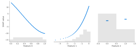
sv_dependence(shap_lm$add, xvars)sv_dependence(shap_lm$add, xvars, color_var = NULL)

shap_lm = {
    "add": shap.Explainer(model_lm.predict, masker=X, algorithm="additive")(X),
    "perm": shap.Explainer(model_lm.predict, masker=X, algorithm="exact")(X),
    "kern": shap.KernelExplainer(model_lm.predict, data=X).shap_values(X),
}

shap_lgb = {
    "tree": shap.Explainer(model_lgb)(X),
    "perm": shap.Explainer(model_lgb.predict, masker=X, algorithm="exact")(X),
    "kern": shap.KernelExplainer(model_lgb.predict, data=X).shap_values(X),
}

# Consistency for additive linear regression
eps = 1e-12
assert np.abs(shap_lm["add"].values - shap_lm["perm"].values).max() < eps
assert np.abs(shap_lm["perm"].values - shap_lm["kern"]).max() < eps

# Consistency for additive boosted trees
assert np.abs(shap_lgb["tree"].values - shap_lgb["perm"].values).max() < eps
assert np.abs(shap_lgb["perm"].values - shap_lgb["kern"]).max() < eps

# Linear effect of last feature in the fitted model
model_lm.named_steps["lm"].coef_[-1]  # 1.112096

# Linear effect of last feature derived from SHAP values (ignore the sign)
shap_lm["perm"][:, 2].values.ptp()    # 1.112096

shap.plots.scatter(shap_lm["add"])

Yes – the three algorithms within model provide the same SHAP values. Furthermore, the SHAP values reconstruct the additive components of the features.

Didactically, this is very helpful when introducing SHAP as a method: Pick a white-box and a black-box model and compare their SHAP dependence plots. For the white-box model, you simply see the additive components, while the dependence plots of the black-box model show scatter due to interactions.

Remark: The exact equivalence between algorithms is lost, when

• there are too many features for exact procedures (~10+ features), and/or when
• the background data of Kernel/Permutation SHAP does not agree with the training data. This leads to slightly different estimates of the baseline value, which itself influences the calculation of SHAP values.

Final words

• SHAP algorithms applied to additive models typically give identical results. Slight differences might occur because sampling versions of the algos are used, or a different baseline value is estimated.
• The resulting SHAP values describe the additive components.
• Didactically, it helps to see SHAP analyses of white-box and black-box models side by side.

R script , Python notebook

Continue reading: SHAP Values of Additive Models

Analysis of SHAP Values of Additive Models

Recent years have seen the rise of SHAP (Shapley Additive Explanations) as the preferred way to investigate black-box models. SHAP’s fundamental premise is to break down model predictions into additive contributions of features in a fair manner. The thorough break down of numerous predictions can uncover global properties of the model.

The application of SHAP to Additive Models

The article proceeds to consider the application of SHAP algorithms to additive models, a concept which, on the face of it, presents an interesting paradox. Analyses are carried out using both high-quality Python and R code, examining model builds using a dataset featuring three significantly correlated covariates and a deterministic response.

Models Built

The authors build additive linear models and additive boosted trees using both R and Python. For both the models, distinct SHAP algorithms have been utilized; Ensuring that the linear model is dissected with additive SHAP and the tree-based model with TreeSHAP.

Are the Results Consistent?

An intriguing question is whether these algorithms would provide similar SHAP values. The answer presented in the paper is a resounding yes. It was demonstrated that individual algorithms yielded the exact SHAP values for each model type. In addition, the SHAP values successfully replicated the additive components of the features.

However, authors noted that there might be a loss in the exact equivalence between the algorithms when there are too many features for exact procedures, or when the background data of Kernel/Permutation SHAP does not agree with the training data. These factors may result in slightly different estimates of the baseline value, which themselves influence the calculation of SHAP values.

Application of SHAP Algorithms to Additive Models: The Implications

For SHAP algorithms applied to additive models, the results are generally identical. Only slight differences might show up if sampling versions of the algorithms are used or if a different baseline value is estimated. These SHAP values describe the additive components, proving the intrinsic value of SHAP as a teaching method. Comparing SHAP analyses of white-box and black-box models side by side serves to facilitate better understanding of this concept.

Suggestions and Ideas

1. Further Research: Since SHAP has been identified as a potential candidate to study black-box models, it makes sense to conduct additional research in this field and explore its wider implications.
2. Improving the Algorithms: It is noted that exact equivalence may be lost between algorithms in certain circumstances. Research should focus on remedying these loopholes to attain more accurate results.
3. Educational Applications: The study proves the didactic value of SHAP for understanding white-box and black-box models. This can form a crucial part of curriculum design in data science and viably be used as a teaching method.
4. Model Comparison: The paper suggests a direct comparison between the SHAP values of white-box and black-box models. This could be a crucial process in future model development and analyses, leading to more robust modelling methodologies.

Conclusion

The study of SHAP values in addictive models offers compelling insights into the investigation of black-box models. As researchers continue to explore this field, we can anticipate a wealth of advanced developments and improved capacities for analyzing complex data models.

Read the original article