ChatGPT has expanded beyond mere textual use cases to incorporate facets of image data and Business Intelligence.
ChatGPT’s Evolution Expanding Beyond Text – Charting Future Trends
In a remarkable reciprocal transformation, OpenAI’s ChatGPT has now grown beyond just text-based functioning. The hefty implications of this pivotal development point towards an AI-present future where machine learning will shape practical applications including but not limited to image data handling and business intelligence.
Long-Term Implications
The move to incorporate image data and business intelligence into the working sphere of ChatGPT marks a crucial expansion in the realm of AI. The implications and the opportunities that this innovative leap brings are manifold:
Innovation in Image Data Handling: With an advanced learning model capable of understanding and processing image data, we might look at a future where AI could read, interpret, and act based on visual inputs. This could reinvent industries, especially those that work extensively with visual data like healthcare, design, security, surveillance, etc.
Better Business Intelligence: An AI with sophisticated analytical capabilities could augment Business Intelligence (BI). This would mean more efficient data collection, improved analytics, sharper forecasts, and more in-depth insights. This will inevitably lead to more intelligent decision-making and supply chain optimization.
Potential Future Developments
There are a multitude of exciting future possibilities following this expansion of ChatGPT:
New Tools for Creative Professionals: More efficient and user-friendly tools for design professionals could be one of the benefits. AI could be used for everything from understanding design briefs to providing creative direction. This could drastically reduce the time otherwise taken in repetitive tasks in the creative process.
Enhanced Medical Imaging: AI could read and interpret medical images, helping to identify any abnormalities swiftly and accurately. This could significantly revolutionize diagnostic medicine.
Futuristic Security Systems: Security systems could take an enormous leap, with advanced AI capable of identifying and interpreting images or behaviors to detect potential threats. This could lead to faster and better responses in potential security breaches.
Actionable Insights
Given these implications, it would be prudent for businesses across sectors to respond proactively. Here are some ways of doing so:
Invest in AI Research: Given the promising developments in AI, investment in AI research could be a strategic move for businesses. This would help them in staying ahead in the competitive market and improvise their existing operational procedures.
Upskill Employees: As AI becomes more prevalent, the workforce needs to adapt to maximize these new tools. Businesses should invest in upskilling employees to function in a more AI-driven landscape.
Prepare For Transition: Organizations should start planning for a seamless transition, given the inevitable AI integration in aspects ranging from administrative tasks to complex analytical operations. This would result in a considerable change in how businesses function.
Wrapping Up
The potential for image data and Business Intelligence in ChatGPT is enormous. As this technology develops, businesses and individuals would do well to adapt to these changes. Understanding these implications and acting proactively would be the key to survival and growth in a largely AI-shaped future.
Want to share your content on R-bloggers? click here if you have a blog, or here if you don’t.
I messed around with DBI and RSQLite and learned it’s actually pretty simple to use in R – just connect, write tables, and use SQL queries without all the complicated server stuff. Thanks to Alec Wong for suggesting this!
Motivation
After our last blog, my friend Alec Wong suggested that I switch storing data from CSV files to SQLite when building Plumber API. I had no idea that CSV files can get corrupted when multiple users hit the API at the same time! SQLite handles this automatically and lets you validate your data without needing to set up any complicated server stuff. It’s actually pretty straightforward, here is a note to myself of some simple and frequent functions.
library(DBI)
library(RSQLite)
library(tidyverse)

con <- dbConnect(drv = RSQLite::SQLite(), "test.sqlite")
That’s it! If the file does not exist, it will create one.
List Tables
Let’s write an sample dataframe and write to a table on the database
# example df
employees <- tibble(
  name = c("John Doe", "Jane Smith", "Bob Johnson", "Alice Brown"),
  department = c("IT", "HR", "Finance", "Marketing"),
  salary = c(75000, 65000, 80000, 70000)
)

# write df to dataframe
dbWriteTable(conn = con, name = "employees", value = employees)

# See What talbes are in the database
tables <- dbListTables(con)
tables

## [1] "employees"
Pretty straightforward!
Check Data
## Method 1
employees_db <- tbl(con, "employees")
employees_db |> collect()

## # A tibble: 4 × 3
##   name        department salary
##   <chr>       <chr>       <dbl>
## 1 John Doe    IT          75000
## 2 Jane Smith  HR          65000
## 3 Bob Johnson Finance     80000
## 4 Alice Brown Marketing   70000
Have to use collect to return a df. We can also do this instead
## Method 2
dbGetQuery(con, "select * from employees")

##          name department salary
## 1    John Doe         IT  75000
## 2  Jane Smith         HR  65000
## 3 Bob Johnson    Finance  80000
## 4 Alice Brown  Marketing  70000
Add Data
## Create New Row of Data
new_employee <- data.frame(
  name = "Sarah Johnson",
  department = "Research",
  salary = 78000
)

## Write to existing table
dbWriteTable(conn = con, name = "employees", value = new_employee, append = TRUE)

tbl(con, "employees") |> collect()

## # A tibble: 5 × 3
##   name          department salary
##   <chr>         <chr>       <dbl>
## 1 John Doe      IT          75000
## 2 Jane Smith    HR          65000
## 3 Bob Johnson   Finance     80000
## 4 Alice Brown   Marketing   70000
## 5 Sarah Johnson Research    78000
Dataframe must contain the same column names and number. Else, won’t work
## New column
new_employee <- data.frame(
  name = "Sarah Johnson",
  department = "Research",
  salary = 78000,
  something_new = 12321321
)

dbWriteTable(con, "employees", value = new_employee, append = T)
# OR
# dbAppendTable(con, "employees", new_employee)

Error: Columns `something_new` not found
Query Data
Filter
dbGetQuery(con, "select * from employees where department = 'Research'")

##            name department salary
## 1 Sarah Johnson   Research  78000
Filter With Matching Operator
dbGetQuery(con, "select * from employees where name like '%john%'")

##            name department salary
## 1      John Doe         IT  75000
## 2   Bob Johnson    Finance  80000
## 3 Sarah Johnson   Research  78000
notice that it’s case insensitive when we use like.
dbGetQuery(con, "select * from employees where name like 's%'")

##            name department salary
## 1 Sarah Johnson   Research  78000
Group Department and Return Average Salary
dbGetQuery(con, "select department, avg(salary) as avg_salary
           from employees
           group by department")

##   department avg_salary
## 1    Finance      80000
## 2         HR      65000
## 3         IT      75000
## 4  Marketing      70000
## 5   Research      78000
Sum Salary With New Column Name
dbGetQuery(con, "select sum(salary) as total_salary from employees")

##   total_salary
## 1       368000
Count Number of Departments
dbGetQuery(con, "select count(distinct department) as distinct_department
           from employees")

##   distinct_department
## 1                   5
Using glue_sql
var <- c("name","department")
table <- "employees"
query <- glue::glue_sql("select {`var`*} from {`table`}", .con = con)
dbGetQuery(con, query)

##            name department
## 1      John Doe         IT
## 2    Jane Smith         HR
## 3   Bob Johnson    Finance
## 4   Alice Brown  Marketing
## 5 Sarah Johnson   Research
Notice the asterisk (*) after {var} – this tells glue_sql() to join the elements with commas automatically. glue_sql provides an f-string feel to the code.
Remove Data
## Delete Using Filter
dbExecute(con, "delete from employees where name = 'Sarah Johnson'")

## [1] 1

dbGetQuery(con, "select * from employees")

##          name department salary
## 1    John Doe         IT  75000
## 2  Jane Smith         HR  65000
## 3 Bob Johnson    Finance  80000
## 4 Alice Brown  Marketing  70000
Remove With Filter
dbGetQuery(con, "select * from employees")

##          name department salary
## 1    John Doe         IT  75000
## 2  Jane Smith         HR  65000
## 3 Bob Johnson    Finance  80000
## 4 Alice Brown  Marketing  70000

dbExecute(con, "delete from employees where salary >= 75000 and department = 'Finance'")

## [1] 1

dbGetQuery(con, "select * from employees")

##          name department salary
## 1    John Doe         IT  75000
## 2  Jane Smith         HR  65000
## 3 Alice Brown  Marketing  70000
Notice how = requires case sensitive F on Finance to filter accurately? Bob no longer in dataframe!
Disconnect
dbDisconnect(con)
Acknowledgement
Thanks again to Alec for suggesting improvements on our previous project!
Understanding DBI and RSQLite: Key Insights and Future Developments
The initial analysis revealed the ease of using DBI and RSQLite in R without dealing with all the complicated server concepts. The key motivation behind this transition was driven by Alec Wong’s suggestion to switch from storing data in CSV files to SQLite when building Plumber API. The key findings revealed that CSV files can easily get corrupted when multiple users access the API simultaneously. SQLite effectively manages this through automatic validation of your data, without necessitating any complex server setup.
Long-term Implications
In the long term, the SQLite adoption can enhance data handling in various ways. SQLite is capable of handling multiple users without any data corruption problems. Moreover, SQLite allows easy data validation without the need for a complicated server setup. Future API building or other data storing tasks may increasingly choose to use systems such as SQLite over traditional options like CSV to enhance data security and ease of use.
Potential Future Developments
As more people discover the benefits of SQLite, there may be further improvements and developments in this area. The future may see an increase in functions and procedures that provide even greater ease in data management and query execution. Furthermore, as data integrity and security become more prevalent concerns, techniques such as SQLite can be expected to become integral parts of most data management processes.
Actionable Advice
If you’re considering a migration from CSV files to SQLite, it’s advisable to get comfortable with SQL as this will be a primary requirement for using SQLite. It might also be beneficial to add this to your pressure logger for even more efficient data handling. Depending on your specific needs, you could add it within the same database even in a different table.
Exploring the Procedures
Several operations, ranging from connecting to a database, checking data, adding data, querying data, removing data and disconnecting from a database were performed. The data was neatly organized into easy-to-understand tables making SQLite handling in R a smooth process. Specific code snippets showcasing the different functions executed have been provided for reference.
Conclusion
In conclusion, switching to SQLite from CSV files for storing data when building a Plumber API has numerous benefits such as preventing file corruption from multiple simultaneous accesses and allowing data validation without complex server settings. Learning and enhancing SQL skills are prerequisites to fully leverage the benefits of SQLite and other similar systems.
These oddball Python functions might seem pointless… until you realize how surprisingly useful they really are.
The Curious Power of Python’s Oddball Functions
As those familiar with Python will already know, the language is filled with a wide range of functionalities. From the simple to the complex, from the familiar to the downright bizarre. None of these are more fascinating than Python’s collection of oddball functions. They may seem irrelevant at first, yet they hold an unanticipated utility that can truly expedite the coding process.
The Long-Term Implications and Future Developments
Python, due to its elegance and simplicity, has become a dominant force in the world of programming, especially in the fields of Data Science and Machine Learning. The use of Python’s oddball functions can enhance productivity by allowing users to perform tasks more efficiently and effectively.
Even though these functions seem to be a bit odd or pointlessly complex, their real-world application extends to various fields. As the use of Python grows, it can be anticipated that the need for more unusual, but highly useful, tools in its armoury will become apparent.
For example, more businesses are harnessing the power of Big Data and Artificial Intelligence. The number of Python applications in these areas will likely increase due to the flexibility of Python and its compelling feature set. In this context, the so-called oddball functions provide Python an advantage over competing languages, possessing the ability to execute quirky code solutions that makes it more adaptable to emerging technological trends.
Actionable Advice
To make the most of Python’s set of oddball functions, one must first stay open to continually learning about Python’s capabilities. However, without contextual examples, it’s tough to see the value of these functions. Hence, it’s recommended to seek out diverse coding problems that could be solved using these rare jewels.
Embrace the unfamiliar: Don’t shy away from the strange and unique functions within Python. They may be unusual, but their usefulness is beyond doubt. Delve into them, understand their role, and attempt to use them regularly in your coding practices.
Constant Learning: Programming languages, like Python, are constantly evolving. Keep yourself updated with the latest Python releases, improvements, and updates.
Practical Application: Theory and practice go hand in hand. The more you use these oddball functions in real-life projects, the more familiar and useful they will become.
At first, these oddball functions can feel like they are only complicating the Python language. However, once you understand their value, they can be extremely beneficial, providing a faster, more efficient coding experience.
Remember, discovery is the key to becoming well-versed in any programming language. Pursue exploration of Python’s oddball functions, and you might be pleasantly surprised by their utility in your coding journey.
As a reliable AWS development company, We offer AWS cloud application development, migration, consulting, cloud BI & analytics, and managed cloud services on AWS.
The Future of AWS Development and its Long-Term Implications
Amazon Web Services (AWS) has been making substantial strides in cloud computing technology, offering robust and versatile development, consulting, migration, cloud BI & analytics, and managed cloud services. The consequent long-term implications and future predictions for this growing sector are indeed exciting and poised for profound innovation.
Potential Future Developments
AWS Cloud Application Development: With advancements in cloud platforms, the possibilities for customizable and scalable application development will continue to expand. We will likely see further advancements in serverless computing and container technologies.
AWS Migration: As an increasing number of businesses, small and large, migrate to the cloud, AWS could increase its scope to facilitate easier and more efficient migration strategies.
AWS Consulting: Given the ever-evolving cloud technology environment, labs, consulting, and management services will be in heightened demand to assist businesses in leveraging AWS’ comprehensive features optimally.
Cloud BI & Analytics: With AWS at the forefront, improved data management and streamlined business intelligence processes are on the horizon. AWS will likely continue to advance in data analytics capabilities, thereby enhancing business decision-making.
Managed Cloud Services on AWS: As the number of companies relying on AWS grows, AWS may further enhance its managed cloud services, ensuring peak performance, security, and cost-efficiency.
Long-Term Implications
The AWS development and its encompassing services’ consistent growth have hinted at several long-term implications. The shift to cloud-based services should drive the global digital transformation further, facilitating operational efficiency, flexibility, and scalability for businesses of all sizes. Moreover, with AWS’s robust cloud BI and analytics tools, more data-driven, insightful decision-making for businesses is anticipated.
Actionable Advice
Staying competitive in the digital age requires leveraging the latest technology. Here’s how to use AWS to your benefit:
Consider Cloud Migration: If you haven’t migrated to the cloud yet, evaluate the potential benefits that AWS could offer. Reduced IT costs, scalability, flexibility, and improved security are among the many possible benefits.
Capitalize on AWS Consulting Services: Consult with AWS specialists to fully realize its potential. They can guide your cloud strategy, provide expert architectural guidance, and offer advice based on specific business needs.
Evolve with Cloud BI & Analytics: Harness AWS’s advanced BI & analytics tools for enhanced, data-informed decision making. From data warehousing to business intelligence, dive into the insights made possible with AWS.
Consider Managed Cloud Services: Managed services can help you navigate the complexities of AWS and ensure your systems are always functioning optimally. It can also help you save costs over DIY AWS management.
As technology continues to progress, adopting and adapting to new tools like AWS are integral to a business’s success.
[This article was first published on Getting Genetics Done, and kindly contributed to R-bloggers]. (You can report issue about the content on this page here)
Want to share your content on R-bloggers? click here if you have a blog, or here if you don’t.
Faster package installation, import only the functions you want with use(), built-in Palmer penguins data, grep values shortcut, and lots of new bioinformatics packages in Bioconductor
…
R 4.5.0 was released last week, and Bioconductor 3.21 came a few days later. You can read the R release notes here and the Bioconductor 3.21 announcement here. Here I’ll highlight a few things that are worth upgrading for.
Any time the minor version changes (e.g., 4.4.x to 4.5.x) you’ll need to reinstall all your packages again. Which will now be much faster thanks to under-the-hood changes to install.packages() that downloads packages in parallel:
install.packages() and download.packages() download packages simultaneously using libcurl, significantly reducing download times when installing or downloading multiple packages.
I don’t have any benchmarks to show but I can tell you reinstalling all my go-to packages was much faster than with previous upgrades and reinstalls.
I keep my own “verse” package on GitHub: github.com/stephenturner/Tverse. This “package” is just an empty package with a DESCRIPTION listing all the packages I use most frequently as dependencies (tidyverse, janitor, pkgdown, usethis, breakerofchains, knitr, here, etc). I’ll first install.packages("devtools"), then devtools::install_github("stephenturner/Tverse"), and all the packages I use most frequently are installed because this dummy “verse” package depends on them. You never want to load this library, but it’s an easy way to reinstall all the R package you use frequently on any new machine or with an R upgrade.
Built-in penguins data
The built-in iris dataset leaves something to be desired. It’s overused and not very engaging for learners or audiences who’ve seen it repeatedly. It’s small (150 rows), clean (no missing data), and doesn’t present challenges to deal with like outliers and multiple categorical labels. And, if you look at the help for ?iris, you’ll see it was published by Ronald Fisher in the Annals of Eugenics, not something I’d care to cite.
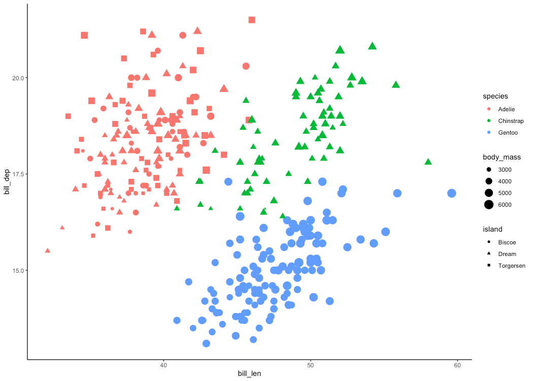
Back in 2020, Allison Horst published the palmerpenguins package — a data package meant to provide a great dataset for data exploration and visualization as an alternative to iris. Previously you had to install the package to use the data, but now the penguins data is built in, as is the less clean penguins_raw data that can be used for teaching data cleaning and manipulation.
And if you’ve written tutorials using the palmerpenguins package, know that the column names differ between the palmerpenguins and base R versions. You might check out the new basepenguins package (documentation). This package gives you functions to convert all your code over to use the base version.
Import only what you want with use()
If you’re coming from Python you’re used to being able to only import what you need from installed packages. E.g.:
from numpy import array, mean
from pathlib import Path
With R if you want to call a function from a package without loading the entire namespace you can always use the double-colon, e.g. dplyr::select(). With R 4.5.0 you can import only the functions you want from any particular package.
use("dplyr", c("filter", "count"))
penguins |>
  filter(island=="Torgersen" & year==2007) |>
  count(sex)
     sex n
1 female 8
2   male 7
3   <NA> 5
There’s a gotcha here though. As the documentation states, use() is a simple wrapper around library which always uses attach.required=FALSE. That means once you call use() the first time, you need to import all of the functions that you might want to import. If you call use() again or even library(), you still won’t have access to those other functions.
In reality I think I’ll still use the package::function() syntax when I don’t want to load the full library, but it’s nice to have this option. See also the box and conflicted packages.
## This works
use("dplyr", c("filter", "count"))
penguins |>
  filter(island=="Torgersen" & year==2007) |>
  count(sex)

## This fails!
library(dplyr)
penguins |>
  mutate(ratio=bill_len/bill_dep)
Error in mutate(penguins, ratio = bill_len/bill_dep) :
  could not find function "mutate"
grepv(): shortcut for grep(..., value=TRUE)
A very small quality of life improvement. If you use grep(), you get the indices of the vector that match your pattern. To get the actual matched values, you can add value=TRUE, or just use the new grepv() function instead.
if (!require("BiocManager", quietly = TRUE))
    install.packages("BiocManager")
BiocManager::install(version = "3.21")
There are 72 new software packages in this release of Bioconductor, bringing the total 2341 software packages, 432 experiment data packages, 928 annotation packages, 30 workflows and 5 books. This release introduces a wide array of new tools and packages across genomics, transcriptomics, proteomics, metabolomics, and spatial omics analysis. Notable additions include new frameworks for spatial transcriptomics (like clustSIGNAL, SEraster, and CARDspa), enhanced utilities for analyzing single-cell data (SplineDV, mist, dandelionR), and cutting-edge methods for integrating and visualizing multi-omics datasets (RFLOMICS, pathMED, MetaboDynamics). The release also features robust statistical and machine learning approaches, such as LimROTS, CPSM, and XAItest, for improved inference and predictive modeling. Several tools improve visualization, accessibility, and reproducibility, including GUI-based apps (geyser, miaDash, shinyDSP) and packages focused on optimizing performance or interoperability (e.g., RbowtieCuda, ReducedExperiment, Rigraphlib).
You may also want to skim through the release notes to look through the updates to existing packages you already use.
To leave a comment for the author, please follow the link and comment on their blog: Getting Genetics Done.
Long-term Implications and Future Developments for R 4.5.0 and Bioconductor 3.21
The release of R 4.5.0 and Bioconductor 3.21 have significant long-term implications for the field of data science, particularly in the realm of bioinformatics. This article will explore the merits of these updates and discuss potential future developments.
Faster Package Installation
R 4.5.0 boasts significantly enhanced package installation speeds. The minor version change has initiated technical alterations that enable install.packages() to download packages in parallel. Users can expect much faster download times when installing or downloading multiple packages, thereby streamlining project setup.
Actionable advice: Maintaining a ‘verse’ package that lists frequently used packages as dependencies is an efficient way to reinstall all necessary packages on a new machine or following an R upgrade. Maintain and update your ‘verse’ package to continually streamline your workflow.
Useful Data for Learning
The addition of the built-in penguins data to R 4.5.0 provides more engaging and diverse data for learners. Unlike the iris dataset, which is overused and lacks challenges like outliers and multiple categorical labels, the penguins dataset offers a more realistic basis for data exploration and visualization training.
Actionable advice: For those writing tutorials, familiarize yourself with the built-in penguins data and consider using it to offer a more stimulating learning environment.
Import Only the Functions You Want with use()
The use() function in R 4.5.0 allows users to import only the functions they need from installed packages. However, once you use the function, you will need to import all the functions you might want to import as trying to import other functions later will not be possible.
Actionable advice: Learn and implement the use of use() judiciously to optimize your workspace.
New Package: Bioconductor 3.21
Bioconductor 3.21 offers 72 new software packages, enhancing the analytical capabilities of genomics, transcriptomics, proteomics, metabolomics, and spatial omics. Tools for spatial transcriptomics, single-cell data analysis, multi-omics datasets integration, robust statistical and machine learning approaches, and improved visualization are some of the impactful offerings.
Actionable advice: Regularly update your version of Bioconductor and familiarize yourself with the latest packages. Bioconductor 3.21’s considerable additions could greatly enhance your data analysis capabilities.
Conclusion
The upgraded releases of R and Bioconductor are steps towards improving productivity, expanding analytical capacities, and enriching the learning process. By integrating the newly added functionalities into their workflows, data scientists and learners can progressively elevate their skills and outcomes. Keeping abreast of these enhancements and understanding how to utilize them will likely be integral to success in future data analysis endeavors.
Try these MCP servers with Claude Desktop today for free.
Analysis of MCP Servers with Claude Desktop
The statement above encourages users to try MCP servers with Claude Desktop for free today. Although not much detail is given, we can glean several key points from this statement to help us predict long-term implications, potential future developments, and to provide actionable advice.
Key Points
There is an integration between MCP servers and Claude Desktop.
This service is currently free.
Long-Term Implications
The integration of MCP servers with Claude Desktop may signify that these two entities are invested in a long-term partnership. This would bring about numerous opportunities for offering combined innovations and upgraded features, as well as potential enterprise-level solutions.
As more services move to the cloud, these types of integrations become increasingly valuable. Companies may look to simplify their operations by using integrated products, as opposed to setting up and maintaining multiple separate systems.
Potential Future Developments
In terms of future developments, we could foresee expanded service offerings, new features, and further integrations. It also stands to reason that pricing models could change as the free trial period concludes. Users may then have the option of various pricing tiers according to their usage and needs.
Actionable Advice
To take full advantage of this offer, users are advised to:
Try the MCP servers with Claude Desktop while the service is still free. This will allow them to assess the benefits and drawbacks before potentially incurring any costs.
Keep an eye on future updates and developments to ensure they are utilizing the service to its full potential. They might also want to explore other products from these providers that could also cater to their business needs.
Offer feedback to the providers. This can help shape future developments and improvements to the service.
Conclusion
While the statement provided is brief, it has significant implications for those interested in leveraging MCP servers and Claude Desktop. Users are advised to maximize the free service period and keep an eye on future developments while also actively providing feedback to optimize their user experience.”