“Examining Fragile P Values: A Closer Look at Research Practices”

by jsendak | Jun 8, 2025 | DS Articles

Do ‘fragile’ p values tell us anything?

I was interested recently to see this article on p values in the psychology literature float across my social media feed. Paul C Bogdan makes the case that the severity of the replication crisis in science can be judged in part by the proportion of p values that are ‘fragile’,which he defines as between 0.01 and 0.05.

Of course, concern at the proportion of p values that are ‘significant but only just’ is a stable feature of the replication crisis. One of the standing concerns with science is that researchers use questionable research practices to somehow nudge the p values down to just below the threshold deemed to be “signficant” evidence. Another standing concern is that researchers who might not use those practices in the analysis themselves will not publish or not be able to publish their null results, leaving a bias towards positive results in the published literature (the “file-drawer” problem).

Bogdan argues that for studies with 80% power (defined as 1 minus the probability of accepting the null hypothesis when there is in fact a real effect in the data), 26% of p values that are significant should be in this “fragile” range, based on simulations.

The research Bogdan describes in the article linked above is a clever data processing exercise of published psychology literature to see what proportion of p values are in fact, “fragile” and how this changes over time. He finds that “From before the replication crisis (2004–2011) to today (2024), the overall percentage of significant p values in the fragile range has dropped from 32% to nearly 26%”. As 26% is about what we’d expect, if all the studies had power of 80%, then this is seen as good news.

Is the replication crisis over? (to be fair, I don’t think Bogdan claims this last point).

One of Bogdan’s own citations is this piece by Daniel Lakens, which itself is a critique of a similar attempt at this earlier. Lakens argues “the changes in the ratio of fractions of p-values between 0.041–0.049 over the years are better explained by assuming the average power has decreased over time” rather than by changes in questionable research practices. I think I agree with Lakens on this.

I just don’t think the 26% of significant p values to be ‘fragile’ is a solid enough benchmark to judge research pracices on.

Anyway, all this intrigued me enough when it was discussed first in Science (as “a big win”) and then on Bluesky for me to want to do my own simulations to see how changes in effect sizes and sample sizes would change that 26%. My hunch was 26% was based on assumptions that all studies have 80% power and (given power has to be calculated for some assumed but unobserved true effect size) that the actual difference in the real world is close to the difference assumed in making that power calculation. Both these assumptions are obviously extremely brittle, but what is the impact if they are wrong?

From my rough playing out below, the impact is pretty material. We shouldn’t think that changes in the proportion of signficant p values that are between 0.01 and 0.05 tells us much about questionable research practices, because there is just too much else going on — pre-calculated power, how much power calculations and indeed the research that is chosen are based on a good reflection of reality, the size of differences we’re looking for, and sample sizes — confounding the whole thing.

Do your own research simulations

To do this, I wrote a simple function experiment which draws two independent samples from two populations, all observations normally distributed. For my purposes the two sample sizes are going to be the same and the standard deviations the same in both populations; only the means differ by population. But this function is set up for a more general exploration if I’m ever motivated.

The ideal situation – researcher’s power calculation matches the real world

With this function I first played around a bit to get a situation where the power is very close to 80%. I got this with sample sizes of 53 each and a difference in the means of the two populations of 0.55 (remembering each population has a standard distribtuion of N(0, 1)).

I then checked this with a published power package, Bulus, M. (2023). pwrss: Statistical Power and Sample Size Calculation Tools. R package version 0.3.1. https://CRAN.R-project.org/package=pwrss. I’ve never used this before and just downloaded it to check I hadn’t made mistakes in my own calculations, and later I will use it to speed up some stuff.

library(pwrss)
library(tidyverse)

experiment <- function(d, m1 = 0, sd1 = 1, sd2 = 1, n1 = 50, n2 = n1, seed = NULL){
  if(!is.null(seed)){
    set.seed(seed)
  }
  x1 <- rnorm(n1, m1, sd1)
  x2 <- rnorm(n2 ,m1 + d, sd2)
  t.test(x1, x2)$p.value
}

reps <- 10000
res <- numeric(reps)

for(i in 1:reps){
  res[i] <- experiment(d = 0.55, n1 = 53)
}

Yes, that’s right, I’m using a for loop here. Why? Because it’s very readable, and very easy to write.

Here’s what that gives us. My simulated power is 80%, Bulus’ package agrees with 80%, and 27% of the ‘signficant’ (at alpha = 0.05) p values are in the fragile range. This isn’t the same as 26% but it’s not a million miles away; it’s easy to imagine a few changes in the experiment that would lead to his 26% figure.

> # power from simulation
> 1 - mean(res > 0.05)
[1] 0.7964
>
> # power from Bulus' package
> pwrss.t.2means(mu1 = 0.55, sd1 = 1, sd2 = 1, n2 = 53)
 Difference between Two means
 (Independent Samples t Test)
 H0: mu1 = mu2
 HA: mu1 != mu2
 ------------------------------
  Statistical power = 0.801
  n1 = 53
  n2 = 53
 ------------------------------
 Alternative = “not equal”
 Degrees of freedom = 104
 Non-centrality parameter = 2.831
 Type I error rate = 0.05
 Type II error rate = 0.199
>
> # Of those experiments that have 'significant' results, what proportion are in
> # the so-called fragile range (i.e. betwen 0.01 and 0.05)
> summ1 <- mean(res > 0.01 & res < 0.05) / mean(res < 0.05)
> print(summ1)
[1] 0.2746107

Changes in difference and in sample size

I made some arbitrary calls in that first run — sample size about 50 observations in each group, and the difference about 0.5 standard deviations. What if I let the difference between the two populations be smaller or larger than this, and just set the number of observations to whatever is necessary to get 80% power? What change does this make to the proportion of p values that are ‘fragile’?

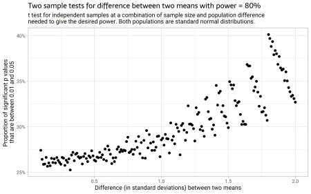
It turns out it makes a big difference, as we see in these two charts:

These are simulations, still in the world where the researcher happens to guess the real world exactly right when they do their power calculation and determine a sample size to get 80% power. We see in the top chart that as the real world difference gets bigger, with constant power, the proportion of significant but ‘fragile’ p values goes up markedly. And the second chart shows the same simulations, but focusing on the variation in sample size which changes in compensation for the real world difference in populations, to maintain the same power. Bigger samples with the same power mean that you are looking for relatively smaller real world differences, and the proportion of significant p values that are ‘fragile’ gets smaller.

Here’s the code that did these simulations:

#--------------varying difference and sample sizes---------------
possible_diffs <- 10:200 / 100 # measured in standard deviations

# what sample size do we need to have 80% power
n_for_power <- sapply(possible_diffs, function(d){
  as.numeric(pwrss.t.2means(mu1 = d, power = 0.8, verbose = FALSE)$n[1])
})

prop_fragile <- numeric(length(possible_diffs))

# This takes some minutes to run, could be better if parallelized or done in
# Julia if we thought saving those minutes was important:
for(j in 1:length(possible_diffs)){
  for(i in 1:reps){
    res[i] <- experiment(d = possible_diffs[j], n1 = n_for_power[j])
  }
  prop_fragile[j] <- mean(res > 0.01 & res < 0.05) / mean(res < 0.05)
}

# Plot 1
tibble(prop_fragile, possible_diffs) |>
  ggplot(aes(x = possible_diffs,y= prop_fragile)) +
  geom_point()+
  scale_y_continuous(label = percent) +
  labs(x = "Difference (in standard deviations) between two means",
       y = "Proportion of significant p values nthat are between 0.01 and 0.05",
       title = "Two sample tests for difference between two means with power = 80%",
       subtitle = "t test for independent samples at a combination of sample size and population differencenneeded to give the desired power. Both populations are standard normal distributions.")

# Plot 2
tibble(prop_fragile, n_for_power) |>
  ggplot(aes(x = n_for_power,y = prop_fragile)) +
  geom_point() +
  scale_x_sqrt() +
  scale_y_continuous(label = percent) +
  labs(x = "Sample size needed to get 80% power for given difference of means",
       y = "Proportion of significant p values nthat are between 0.01 and 0.05",
       title = "Two sample tests for difference between two means with power = 80%",
       subtitle = "t test for independent samples at a combination of sample size and population differencenneeded to give the desired power. Both populations are standard normal distributions.")

Relaxing assumptions

OK, so that was what we get when the power calculation was based on a true representation of the world, known before we did the experiment. Obviously this is never the case (or we’d not need to do experiments) — the actual difference between two populations might be bigger or smaller than we expected, it might actually be exactly zero, the shape and spread of the populations will differ from what we thought when we calculated the power, etc.

I decided to try three simple breaks of the assumptions to see what impact they have on the 27% of p values that were fragile:

• The actual difference between populations is a random number, albeit on average is what is expected during the power calculation
• the actual difference between populations is a coin flip between exactly what was expected (when the power calculation was made) and zero (ie null hypothesis turns out to be true)
• the actual difference between population is a coin flip between a random number with average the same as expected and zero (ie a combination of the first two scenarios)

#------------------when true d isn't what was expected---------------

reps <- 10000
res <- numeric(reps)

# we are going to let the actual difference deviate from that which was used
# in the power calculation, but say that on average the planned-for difference
# was correct
for(i in 1:reps){
  res[i] <- experiment(d = rnorm(1, 0.55, 0.5), n1 = 53)
}

# "actual" power:
1 - mean(res > 0.05)

# proportion of so-called fragile p values is much less
summ2 <- mean(res > 0.01 & res < 0.05) / mean(res < 0.05)

#---------when true d is same as expected except half the time H0 is true---------

for(i in 1:reps){
  res[i] <- experiment(d = sample(c(0, 0.55), 1), n1 = 53)
}


# proportion of so-called fragile p values is now *more*
summ3 <- mean(res > 0.01 & res < 0.05) / mean(res < 0.05)

#---------when true d is random, AND half the time H0 is true---------

for(i in 1:reps){
  res[i] <- experiment(d = sample(c(0, rnorm(1, 0.55, 0.5)), 1), n1 = 53)
}


# proportion of so-called fragile p values is now less
summ4 <- mean(res > 0.01 & res < 0.05) / mean(res < 0.05)

tibble(`Context` = c(
  "Difference is as expected during power calculation",
  "Difference is random, but on average is as expected",
  "Difference is as expected, except half the time null hypothesis is true",
  "Difference is random, AND null hypothesis true half the time"
), `Proportion of p-values that are fragile` = c(summ1, summ2, summ3, summ4)) |>
  mutate(across(where(is.numeric), (x) percent(x, accuracy = 1))) 

That gets us these interesting results:

There’s a marked variation here in what proportion of p values is fragile. Arguably, the fourth of these scenarios is the closest approximation to the real world (although there is a lot of debate about this, how much are exactly-zero differences really plausible?) Either this, or the other realistic scenario (‘difference is random but on average is as expected’) gives a proportion of fragile p values well below the 27% we saw in our base scenario.

Conclusion

There’s just too many factors impacting on the proportion of p values that will be between 0.01 and 0.05 to assume that variations in it are either an improvement or a worsening in research practices. These things include:

• When expected differences change and sample sizes change to go with them for a given level of power, it impacts materially on the proportion of fragile p values we’d expect to see
• When the real world differs from that expected by the researcher when they did their power calculation, it impacts materially on the proportion of fragile p values we’d expect to see
• Anyway, researchers don’t all set their sample sizes to give 80% power, for various reasons, some of them good and some not so good

Final thought — none of the above tells us whether we have a replication crisis or not, and if so if it’s getting better or getting worse. As it happens, I tend to think we do have one and that it’s very serious. I think the peer review process works very poorly and could be improved, and academic publishing in general sets up terrible — and perhaps worsening — incentives. However, I think criticism in the past decade or so has led to improvements (such as more access to reproducible code and data, more pre-registration, general raised awareness), which is consistent really with Bogdan’s substantive argument here. I just don’t think the ‘fragile’ p values are much evidence either way, and if we monitor them at all we should do so with great caution.

Continue reading: Power and ‘fragile’ p-values by @ellis2013nz

Analyzing the Reliability of ‘Fragile’ P Values

There has been an ongoing debate about the reliability of ‘fragile’ p values within the scientific community. The ‘replication crisis’ in science has highlighted concerns about the proportion of p values that are significant but only borderline so. This has been linked to perceived questionable research practices, such as using methods to nudge the p values below the defined threshold for significant evidence. Despite this, the overall proportion of significant p values in the “fragile” range has reportedly dropped from 32% to 26%.

Can ‘Fragile’ P Values Be Trusted?

Questioning the validity of ‘fragile’ p values is a crucial aspect of the ongoing replication crisis in science. If assumptions made for power calculations for studies deviate from the real world, the proportion of p values that are ‘fragile’ can be significantly affected. Changes in the expected differences between groups and deviations from power calculations can impact the proportion of ‘fragile’ p values expected significantly. This would imply that the use of ‘fragile’ p values as evidence of research practices improving or worsening may not be valid.

Long-Term Implications

The existence of a replication crisis within the world of research is broadly agreed upon. There is a growing concern that improper research practices, inappropriate incentives, and a faulty peer review process are leading to the generation of unreliable scientific literature. This crisis could lead to erosion of trust in scientific research, misallocation of resources, and potentially flawed public policies based on inaccurate scientific evidence.

Future Developments

Criticism of the current scientific process has started to result in changes, such as greater access to reproducible code and data, more pre-registration of studies, and increased awareness. However, the scientific community must continue to strive for transparency, improved research practices, and enhanced peer-review processes. Technological advancements, notably the development of artificial intelligence (AI) tools, could potentially aid in improving the process of scientific research.

Actionable Advice

1. Strive for Transparency and Openness: Openness in sharing data, materials, and research methodology will foster trust and allow for easier replication of studies.

2. Employ Better Peer-Review Processes: The peer-review process should be revised to encourage more rigorous reviews and to minimize biases. This could include the use of AI tools to help in identifying errors or inconsistencies.

3. Advocate for Responsible Incentive Structures: Current incentive structures that reward quantity over quality of published research should be re-evaluated to maintain the integrity of scientific research.

4. Improve Research Practices: Stricter guidelines and increased training for researchers can minimize questionable research practices.

5. Avoid Over-reliance on ‘Fragile’ P Values: The scientific community should bear in mind that ‘fragile’ p values may not reliably indicate whether research practices are improving or worsening.

Read the original article